import torch
import torchvision
import fastai.vision.all
import matplotlib.pyplot as plt
import requests Class Activation Map
1. Imports
2. CAM의 구현을 위한 학습
A. DLS
path = fastai.data.external.untar_data(fastai.data.external.URLs.PETS)
fnames = [l for l in (path/'images').ls() if str(l).split('.')[-1] == 'jpg']
def label_func(fname):
if fname[0].isupper():
return 'cat'
else:
return 'dog'dls = fastai.vision.data.ImageDataLoaders.from_name_func(
path = path/'images',
fnames = fnames,
label_func = label_func,
valid_pct = 0.2,
item_tfms = fastai.vision.augment.Resize(512),
bs = 32
)dls.show_batch()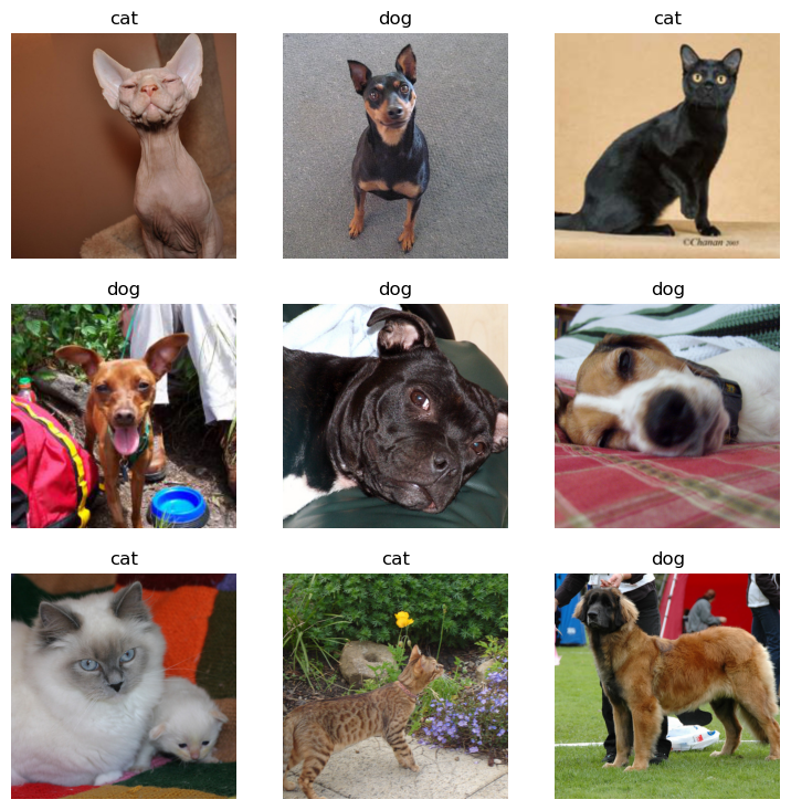
B. 이미지 자료 불러오기
- torchvision 사용
x = torchvision.io.read_image('/root/.fastai/data/oxford-iiit-pet/images/Sphynx_14.jpg')
# x를 찍어보면 int형의 tensor형태로 되어있다
- fastai 사용
path를 이용하는 string \(\to\) PILImage \(\to\) fastai.torch_core.TensorImage \(\to\) torch.tensor
x_pil = fastai.vision.core.PILImage.create('/root/.fastai/data/oxford-iiit-pet/images/Sphynx_14.jpg')
x = next(iter(dls.test_dl([x_pil])))[0]
# x를 찍어보면 float형의 tensor형태로 되어있다
C. 이미지 시각화
x_pil = fastai.vision.core.PILImage.create('/root/.fastai/data/oxford-iiit-pet/images/Sphynx_14.jpg')
x = next(iter(dls.test_dl([x_pil])))[0]
plt.imshow(torch.einsum('ocij -> ijc' , x.to('cpu'))) # cuda에 있으면 시각화가 안 됨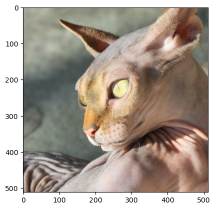
- 아무런 사진이나 하나 가져와서 시각화 해보기
x_pil = fastai.vision.core.PILImage.create(requests.get('https://i.ytimg.com/vi/vc0aaS83cRo/maxresdefault.jpg').content)
x = next(iter(dls.test_dl([x_pil])))[0]
plt.imshow(torch.einsum('ocij -> ijc' , x.to('cpu')))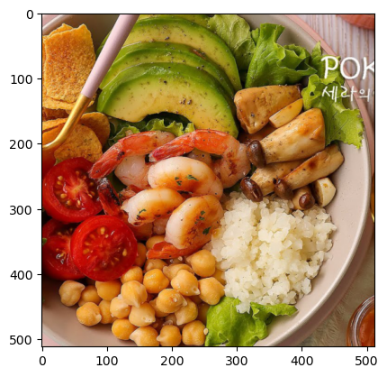
iamge가 잘리는 이유 : dls에서 그림의 size를 512로 정해놨기때문에 512 x 512 image로 출력된다
D. AP layer
ap = torch.nn.AdaptiveAvgPool2d(output_size=1)
apAdaptiveAvgPool2d(output_size=1)X = torch.arange(1*3*4*4).reshape(1,3,4,4)*1.0
Xtensor([[[[ 0., 1., 2., 3.],
[ 4., 5., 6., 7.],
[ 8., 9., 10., 11.],
[12., 13., 14., 15.]],
[[16., 17., 18., 19.],
[20., 21., 22., 23.],
[24., 25., 26., 27.],
[28., 29., 30., 31.]],
[[32., 33., 34., 35.],
[36., 37., 38., 39.],
[40., 41., 42., 43.],
[44., 45., 46., 47.]]]])ap(X) #채널별로 평균을 구해줌tensor([[[[ 7.5000]],
[[23.5000]],
[[39.5000]]]])r,g,b = ap(X)[0]r, g ,b(tensor([[7.5000]]), tensor([[23.5000]]), tensor([[39.5000]]))5. CAM
A. 1단계 - 이미지분류 잘하는 네트워크 선택 후 학습
lrnr = fastai.vision.learner.vision_learner(
    dls = dls,
    arch = fastai.vision.models.resnet34,
    metrics = [fastai.metrics.accuracy]
)lrnr.fine_tune(1) #lrnr.model의 마지막 부분만 학습시키는 걸 fine_tune이라고 함| epoch | train_loss | valid_loss | accuracy | time |
|---|---|---|---|---|
| 0 | 0.087281 | 0.012028 | 0.995940 | 00:19 |
| epoch | train_loss | valid_loss | accuracy | time |
|---|---|---|---|---|
| 0 | 0.051851 | 0.010260 | 0.996617 | 00:26 |
B. 2단계 - 네트워크 부분 수정 후 재학습
net1 = lrnr.model[0]
net2 = lrnr.model[1]
net2 = torch.nn.Sequential(
torch.nn.AdaptiveAvgPool2d(output_size=1),
torch.nn.Flatten(),
torch.nn.Linear(512,2,bias=False)
)net = torch.nn.Sequential(
net1,
net2
) # 내가 만든(수정한) netlrnr2 = fastai.learner.Learner(
dls = dls,
model = net,
metrics = [fastai.metrics.accuracy]
) # 나만의 net으로 새롭게 학습할 lrnr2lrnr.loss_func , lrnr2.loss_func # 정의하지 않아도 알아서 잘 들어가 있다(FlattenedLoss of CrossEntropyLoss(), FlattenedLoss of CrossEntropyLoss())lrnr2.fine_tune(5)| epoch | train_loss | valid_loss | accuracy | time |
|---|---|---|---|---|
| 0 | 0.392073 | 0.295664 | 0.876861 | 00:26 |
| epoch | train_loss | valid_loss | accuracy | time |
|---|---|---|---|---|
| 0 | 0.192747 | 0.190745 | 0.916779 | 00:26 |
| 1 | 0.180415 | 0.234511 | 0.912720 | 00:26 |
| 2 | 0.136703 | 0.168526 | 0.926252 | 00:26 |
| 3 | 0.057196 | 0.052161 | 0.975643 | 00:26 |
| 4 | 0.033394 | 0.049159 | 0.979702 | 00:26 |
C. 3단계 - 수정된 net2에서 linear 와 AP의 순서를 바꿈
x_pil = fastai.vision.core.PILImage.create('/root/.fastai/data/oxford-iiit-pet/images/Sphynx_14.jpg')
x = next(iter(dls.test_dl([x_pil])))[0]
x_dec = dls.decode([x])[0]
plt.imshow(torch.einsum('ocij -> ijc', x_dec))
net2 순서 바꾸기 전 네트워크 진행
ap = lrnr2.model[-1][0]
fl = lrnr2.model[-1][1]
l = lrnr2.model[-1][2]
l(fl(ap(net1(x)))) # 고양이!!TensorImage([[ 2.5441, -2.8503]], device='cuda:0', grad_fn=<AliasBackward0>)- net2 순서 바꾼 후 네트워크 진행
ap = lrnr2.model[-1][0]
fl = lrnr2.model[-1][1]
l = lrnr2.model[-1][2]1. 일단 net1(x)을 진행
2. Linear를 먼저 해야하니 행렬곱
3. ap
4. flatten
flttn(ap(torch.einsum('ocij,kc -> okij' , net1(x) , l.weight.data))) #고양이!!!TensorImage([[ 2.5441, -2.8503]], device='cuda:0', grad_fn=<AliasBackward0>)- 그런데 왜 순서 바꾸는 거지..? 그냥 하면 안돼?
- 순서를 바꾸면 데이터의 차원이 [1,2,?,?] 이런식으로 바뀌는데 2인 부분을 고양이 or 강아지 이런식으로 데이터를 바라볼 수 있다
D. 잠깐… 인공지능이 뭘 보고 고양이인지 강아지인지 구분하는 거지?
WHY = torch.einsum('ocij,kc -> okij',net1(x),l.weight.data)
WHY[0,0,:,:].int()
TensorImage([[ 0, 0, 0, 0, 0, 0, 0, 0, 0, 0, 0, 0, 0, 0, 0, 0],
[ 0, 0, 0, 0, 0, 0, 0, 0, 0, 0, 0, 0, 0, 0, 0, 0],
[ 0, 0, 0, 1, 1, 0, 0, 0, 0, 0, 0, 0, 0, 0, -1, -2],
[ 0, 0, 0, 0, 0, 0, 0, 0, 0, 0, 0, 0, 0, 0, 0, 0],
[ 0, 0, 0, 0, 0, 0, 0, 0, 0, 0, 0, 0, 0, 0, 0, 0],
[ 0, 0, 0, 0, 0, 0, 3, 11, 16, 12, 4, 0, 0, 0, 0, 0],
[ 0, 0, 0, 0, 0, 0, 7, 26, 39, 29, 9, 0, 0, 0, 0, 0],
[ 0, 0, 0, 0, 0, 0, 9, 34, 53, 37, 10, 0, 0, 0, 0, 0],
[ 0, 0, 0, 0, 0, 0, 7, 27, 39, 28, 9, 0, 0, 0, 0, 0],
[ 0, 0, 0, 0, 0, -1, 3, 10, 15, 10, 3, 1, 1, 0, 0, 0],
[ 0, 0, 0, 0, 0, 0, 2, 4, 4, 2, 0, 0, 0, 0, 1, 0],
[ 0, 0, 0, 0, 0, 0, 4, 6, 8, 3, 0, 0, 1, 1, 1, 1],
[ 0, 0, 0, 0, 1, 1, 2, 8, 11, 4, 0, 0, 0, 1, 1, 0],
[ 0, 0, 0, 0, 0, 0, 2, 6, 7, 4, 0, 0, 0, 0, 0, 0],
[ 0, 0, 0, 0, 0, 0, 1, 2, 2, 1, 0, 0, 0, 0, 0, 0],
[ 0, 0, 0, 0, 0, 0, 0, 1, 0, 0, 0, 0, 0, 0, 0, 0]],
device='cuda:0', dtype=torch.int32)- 가운데 쪽에 숫자들이 크다. 저 의미는 인공지능이 그림의 저 부분을 보고 고양이라고 판단했다는 의미
WHY[0,1,:,:].int()TensorImage([[ 0, 0, 0, 0, 0, 0, 0, 0, 0, 0, 0, 0, 0,
0, 0, 0],
[ 0, 0, 0, 0, 0, 0, 0, 0, 0, 0, 0, 0, 0,
0, 0, 0],
[ 0, 0, 0, 0, 0, 0, 0, 0, 0, 0, 0, 0, 0,
0, 0, 0],
[ 0, 0, 0, 0, 0, 0, 0, 0, 0, 0, 0, 0, 0,
1, 1, 0],
[ 0, 0, 0, 0, 0, 0, 3, 8, 5, 1, 0, 0, 0,
0, 0, 0],
[ 0, 0, 0, 0, -3, -9, -8, 6, 5, 1, 0, 2, 3,
1, 0, 0],
[ 0, 0, 0, -1, -14, -42, -59, -42, -15, -1, 0, 7, 4,
0, 0, 0],
[ 0, 0, 0, -2, -20, -65, -97, -72, -25, -3, 0, 1, 1,
0, 0, 0],
[ 0, 0, 0, -2, -21, -64, -93, -71, -28, -4, -1, 0, 0,
0, 0, 0],
[ 0, 0, 0, -1, -12, -33, -45, -36, -15, -3, -1, -1, 0,
0, 0, 1],
[ 0, 0, 0, 0, -3, -8, -12, -8, -3, -1, -1, -1, 0,
0, 0, 0],
[ 0, 0, 0, 0, 0, -2, -5, -1, 0, 0, 0, 0, 0,
0, 0, 0],
[ 0, 0, 0, 0, 0, -2, -3, -1, 0, 0, 0, 0, 0,
0, 0, 0],
[ 0, 0, 0, 0, 0, 0, 0, 0, 0, 0, 0, 0, 0,
0, 0, 0],
[ 0, 0, 0, 0, 0, 0, 0, 0, 0, 0, 0, 0, 0,
0, 0, 0],
[ 0, 0, 0, 0, 0, 0, 0, 0, 0, 0, 0, 0, 0,
0, 0, 0]], device='cuda:0', dtype=torch.int32)- 가운데 쪽에 숫자들이 작다. 저 의미는 인공지능이 그림의 저 부분을 보고 고양이가 아니라고 판단했다는 의미
시각화 해보자
WHYCAT = WHY[0,0,:,:].to('cpu').detach()
WHYDOG = WHY[0,1,:,:].to('cpu').detach()
x_dec = dls.decode([x])[0]
fig , ax = plt.subplots(1,3,figsize=(8,4))
ax[0].imshow(torch.einsum('ocij -> ijc',x_dec))
ax[1].imshow(WHYCAT , cmap='magma')
ax[2].imshow(WHYDOG , cmap='magma')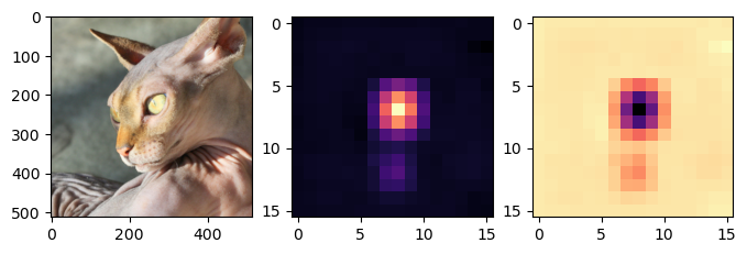
fig ,ax = plt.subplots(1,2,figsize=(8,6))
ax[0].imshow(torch.einsum('ocij -> ijc',x_dec))
ax[0].imshow(WHYCAT , cmap='magma',extent = (0,511,511,0) , interpolation = 'bilinear',alpha=0.5)
ax[1].imshow(torch.einsum('ocij -> ijc',x_dec))
ax[1].imshow(WHYDOG , cmap='magma',extent = (0,511,511,0) , interpolation = 'bilinear',alpha=0.5)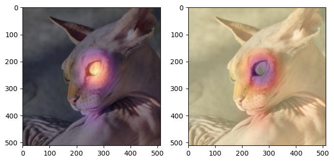
- 주로 눈을 보면서 고양이라고 판단하고 (1번째 그림의 해석) 주로 눈을 보면서 강아지가 아니라고 판단했다(2번째 그림의 해석)
- 다른 사진으로 해보자
x_pil = fastai.vision.core.PILImage.create(requests.get('https://github.com/guebin/DL2024/blob/main/imgs/01wk-hani1.jpeg?raw=true').content)
x = next(iter(dls.test_dl([x_pil])))[0]
x_dec = dls.decode([x])
WHY = torch.einsum('ocij,kc -> okij', net1(x), l.weight.data)
WHYCAT = WHY[0,0,:,:].to("cpu").detach()
WHYDOG = WHY[0,1,:,:].to("cpu").detach()
softmax = torch.nn.Softmax(dim=1)
cat_prob, dog_prob = softmax(flttn(ap(WHY))).to("cpu").detach().tolist()[0]
fig ,ax = plt.subplots(1,2,figsize=(8,6))
ax[0].imshow(torch.einsum('ocij -> ijc',x_dec))
ax[0].imshow(WHYCAT , cmap='magma',extent = (0,511,511,0) , interpolation = 'bilinear',alpha=0.5)
ax[0].set_title(f'cat prob = {cat_prob:.6f}')
ax[1].imshow(torch.einsum('ocij -> ijc',x_dec))
ax[1].imshow(WHYDOG , cmap='magma',extent = (0,511,511,0) , interpolation = 'bilinear',alpha=0.5)
ax[1].set_title(f'dog prob = {dog_prob:.6f}')Text(0.5, 1.0, 'dog prob = 0.999923')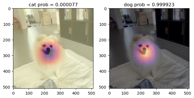
E. 4단계 - CAM 시각화
- 0~25번 사진
fig,ax = plt.subplots(5,5)
k = 0
for i in range(5):
    for j in range(5):
        x_pil = fastai.vision.core.PILImage.create(fnames[k])
        x = next(iter(dls.test_dl([x_pil])))[0]
        x_dec = dls.decode([x])
        WHY = torch.einsum('ocij,kc -> okij', net1(x), l.weight.data)
        WHYCAT = WHY[0,0,:,:].to("cpu").detach()
        WHYDOG = WHY[0,1,:,:].to("cpu").detach()
        cat_prob, dog_prob = softmax(flttn(ap(WHY))).to("cpu").detach().tolist()[0]
        if cat_prob > dog_prob:
            ax[i][j].imshow(torch.einsum('ocij -> ijc', x_dec))
            ax[i][j].imshow(WHYCAT,cmap='magma',extent=(0,511,511,0),interpolation='bilinear',alpha=0.5)
            ax[i][j].set_title(f"cat({cat_prob:.2f})")
            ax[i][j].set_xticks([])
            ax[i][j].set_yticks([])
        else:
            ax[i][j].imshow(torch.einsum('ocij -> ijc', x_dec))
            ax[i][j].imshow(WHYDOG,cmap='magma',extent=(0,511,511,0),interpolation='bilinear',alpha=0.5)
            ax[i][j].set_title(f'dog({dog_prob:.2f})')
            ax[i][j].set_xticks([])
            ax[i][j].set_yticks([])
        k = k+1
fig.set_figheight(16)
fig.set_figwidth(16)
fig.tight_layout()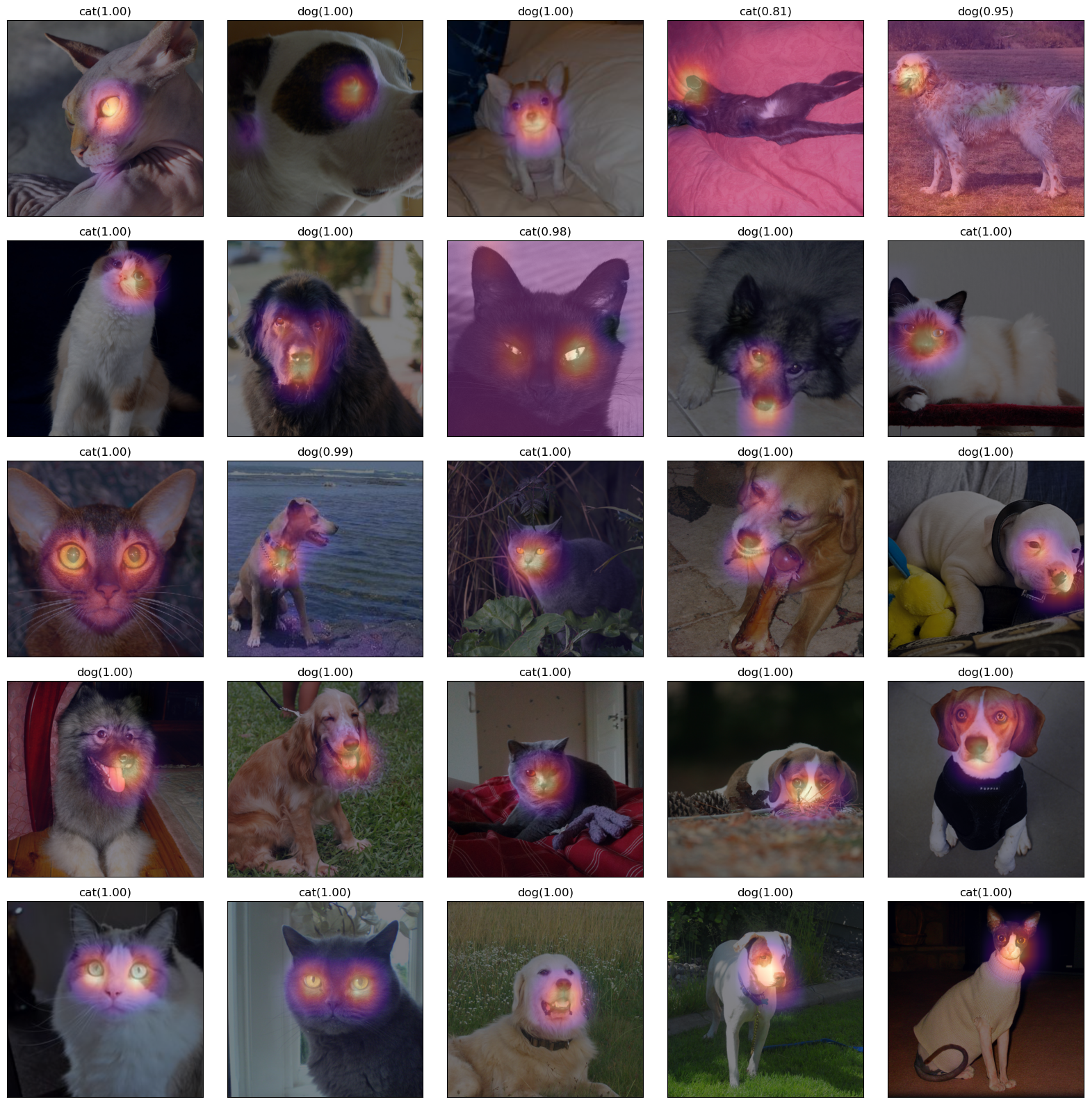
- 26~50번 사진
fig,ax = plt.subplots(5,5)
#---#
k=25
for i in range(5):
    for j in range(5):
        x_pil = fastai.vision.core.PILImage.create(fastai.data.transforms.get_image_files(path/'images')[k])
        x = next(iter(dls.test_dl([x_pil])))[0] # 이걸로 WHY를 만들어보자.
        x_dec = dls.decode([x])[0] # 이걸로 시각화
        WHY = torch.einsum('ocij,kc -> okij',net1(x),l.weight.data)
        WHYCAT = WHY[0,0,:,:].to("cpu").detach()
        WHYDOG = WHY[0,1,:,:].to("cpu").detach()
        cat_prob, dog_prob = softmax(flttn(ap(WHY))).to("cpu").detach().tolist()[0]
        if cat_prob > dog_prob:
            ax[i][j].imshow(torch.einsum('ocij -> ijc',x_dec))
            ax[i][j].imshow(WHYCAT,cmap='magma',extent = (0,511,511,0), interpolation='bilinear',alpha=0.5)
            ax[i][j].set_title(f"cat({cat_prob:.2f})")
            ax[i][j].set_xticks([])
            ax[i][j].set_yticks([])
        else:
            ax[i][j].imshow(torch.einsum('ocij -> ijc',x_dec))
            ax[i][j].imshow(WHYDOG,cmap='magma',extent = (0,511,511,0), interpolation='bilinear',alpha=0.5)
            ax[i][j].set_title(f"dog({dog_prob:.2f})")
            ax[i][j].set_xticks([])
            ax[i][j].set_yticks([])
        k=k+1
fig.set_figheight(16)
fig.set_figwidth(16)
fig.tight_layout() 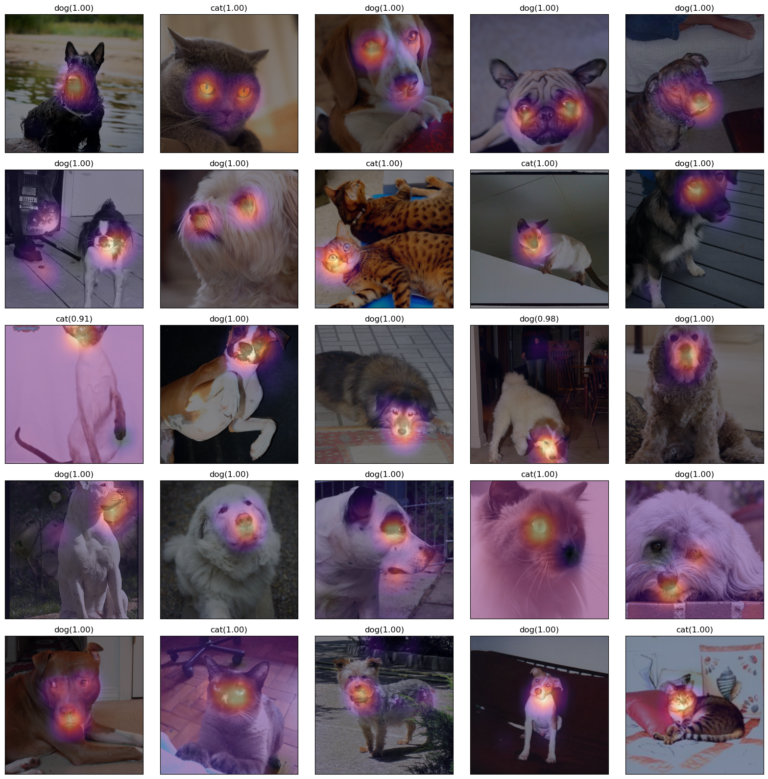
중요 WHY를 만드는 과정에서 Linear는 가중치를 곱하여 더하는 행위이고 행렬곱으로 계산된다.
즉, einsum을 이용하여 계산해주면 된다.
l.weight.data의 값만 바꿔준다면 다른 가중치로도 계산할 수 있다.