About hidden size

1. Imports

import torch
import pandas as pd
import matplotlib.pyplot as plt

soft = torch.nn.Softmax(dim=1)
ohot = torch.nn.functional.one_hot

2. abc

A. Data

txt = list('abc'*100)
txt[:10]

['a', 'b', 'c', 'a', 'b', 'c', 'a', 'b', 'c', 'a']

df_train = pd.DataFrame({'x': txt[:-1], 'y': txt[1:]})
df_train[:5]

x = torch.tensor(df_train.x.map({'a':0,'b':1,'c':2}))
y = torch.tensor(df_train.y.map({'a':0,'b':1,'c':2}))

B. MLP - 하나의 은닉노드

torch.manual_seed(43052)
net = torch.nn.Sequential(
    torch.nn.Embedding(3,1),
    torch.nn.Tanh(), # -1,1사이로 값을 눌러준다
    torch.nn.Linear(1,3), # 피처 뻥튀기 <- 3개 중에 하나를 골라야하기 떄문에.
    # torch.nn.Softmax()
)
loss_fn = torch.nn.CrossEntropyLoss()
optimizr = torch.optim.Adam(net.parameters(),lr=0.1)

for epoc in range(50):
    ## 1 
    netout = net(x) 
    ## 2 
    loss = loss_fn(netout,y)
    ## 3 
    loss.backward()
    ## 4 
    optimizr.step()
    optimizr.zero_grad()

yhat = soft(netout)
yhat.argmax(axis=1),y

(tensor([1, 2, 0, 1, 2, 0, 1, 2, 0, 1, 2, 0, 1, 2, 0, 1, 2, 0, 1, 2, 0, 1, 2, 0,
         1, 2, 0, 1, 2, 0, 1, 2, 0, 1, 2, 0, 1, 2, 0, 1, 2, 0, 1, 2, 0, 1, 2, 0,
         1, 2, 0, 1, 2, 0, 1, 2, 0, 1, 2, 0, 1, 2, 0, 1, 2, 0, 1, 2, 0, 1, 2, 0,
         1, 2, 0, 1, 2, 0, 1, 2, 0, 1, 2, 0, 1, 2, 0, 1, 2, 0, 1, 2, 0, 1, 2, 0,
         1, 2, 0, 1, 2, 0, 1, 2, 0, 1, 2, 0, 1, 2, 0, 1, 2, 0, 1, 2, 0, 1, 2, 0,
         1, 2, 0, 1, 2, 0, 1, 2, 0, 1, 2, 0, 1, 2, 0, 1, 2, 0, 1, 2, 0, 1, 2, 0,
         1, 2, 0, 1, 2, 0, 1, 2, 0, 1, 2, 0, 1, 2, 0, 1, 2, 0, 1, 2, 0, 1, 2, 0,
         1, 2, 0, 1, 2, 0, 1, 2, 0, 1, 2, 0, 1, 2, 0, 1, 2, 0, 1, 2, 0, 1, 2, 0,
         1, 2, 0, 1, 2, 0, 1, 2, 0, 1, 2, 0, 1, 2, 0, 1, 2, 0, 1, 2, 0, 1, 2, 0,
         1, 2, 0, 1, 2, 0, 1, 2, 0, 1, 2, 0, 1, 2, 0, 1, 2, 0, 1, 2, 0, 1, 2, 0,
         1, 2, 0, 1, 2, 0, 1, 2, 0, 1, 2, 0, 1, 2, 0, 1, 2, 0, 1, 2, 0, 1, 2, 0,
         1, 2, 0, 1, 2, 0, 1, 2, 0, 1, 2, 0, 1, 2, 0, 1, 2, 0, 1, 2, 0, 1, 2, 0,
         1, 2, 0, 1, 2, 0, 1, 2, 0, 1, 2]),
 tensor([1, 2, 0, 1, 2, 0, 1, 2, 0, 1, 2, 0, 1, 2, 0, 1, 2, 0, 1, 2, 0, 1, 2, 0,
         1, 2, 0, 1, 2, 0, 1, 2, 0, 1, 2, 0, 1, 2, 0, 1, 2, 0, 1, 2, 0, 1, 2, 0,
         1, 2, 0, 1, 2, 0, 1, 2, 0, 1, 2, 0, 1, 2, 0, 1, 2, 0, 1, 2, 0, 1, 2, 0,
         1, 2, 0, 1, 2, 0, 1, 2, 0, 1, 2, 0, 1, 2, 0, 1, 2, 0, 1, 2, 0, 1, 2, 0,
         1, 2, 0, 1, 2, 0, 1, 2, 0, 1, 2, 0, 1, 2, 0, 1, 2, 0, 1, 2, 0, 1, 2, 0,
         1, 2, 0, 1, 2, 0, 1, 2, 0, 1, 2, 0, 1, 2, 0, 1, 2, 0, 1, 2, 0, 1, 2, 0,
         1, 2, 0, 1, 2, 0, 1, 2, 0, 1, 2, 0, 1, 2, 0, 1, 2, 0, 1, 2, 0, 1, 2, 0,
         1, 2, 0, 1, 2, 0, 1, 2, 0, 1, 2, 0, 1, 2, 0, 1, 2, 0, 1, 2, 0, 1, 2, 0,
         1, 2, 0, 1, 2, 0, 1, 2, 0, 1, 2, 0, 1, 2, 0, 1, 2, 0, 1, 2, 0, 1, 2, 0,
         1, 2, 0, 1, 2, 0, 1, 2, 0, 1, 2, 0, 1, 2, 0, 1, 2, 0, 1, 2, 0, 1, 2, 0,
         1, 2, 0, 1, 2, 0, 1, 2, 0, 1, 2, 0, 1, 2, 0, 1, 2, 0, 1, 2, 0, 1, 2, 0,
         1, 2, 0, 1, 2, 0, 1, 2, 0, 1, 2, 0, 1, 2, 0, 1, 2, 0, 1, 2, 0, 1, 2, 0,
         1, 2, 0, 1, 2, 0, 1, 2, 0, 1, 2]))

C. 적합결과의 해석

- 네트워크 분해

ebdd , tanh , linr = net

- ebdd 레이어 통과 직후

ebdd_x = ebdd(x).data[:9]
ebdd_x

tensor([[ 0.0287],
        [ 1.8616],
        [-2.8092],
        [ 0.0287],
        [ 1.8616],
        [-2.8092],
        [ 0.0287],
        [ 1.8616],
        [-2.8092]])

plt.plot(ebdd_x, '--o', color='gray')
plt.title(r"$ebdd({\bf x})$")
plt.title(r"$ebdd({\bf x})$")
plt.xticks(range(9),[r'$a\to b$', r'$b\to c$', r'$c\to a$']*3);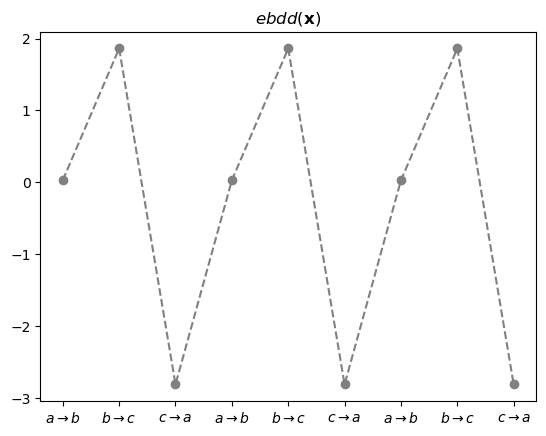

- ebdd -> tanh 레이어 통과 직후

ebdd_x = ebdd(x).data[:9]
h = tanh(ebdd(x)).data[:9]
torch.concat([ebdd_x,h],axis=1)

tensor([[ 0.0287,  0.0287],
        [ 1.8616,  0.9528],
        [-2.8092, -0.9928],
        [ 0.0287,  0.0287],
        [ 1.8616,  0.9528],
        [-2.8092, -0.9928],
        [ 0.0287,  0.0287],
        [ 1.8616,  0.9528],
        [-2.8092, -0.9928]])

fig,ax = plt.subplots(2,1,figsize=(8,8))
ax[0].plot(ebdd_x, '--o', color='gray')
ax[0].set_title(r"$ebdd({\bf x})$")
ax[0].set_xticks(range(9),[r'$a\to b$', r'$b\to c$', r'$c\to a$']*3)
ax[1].plot(h, '--o', color='gray')
ax[1].set_title(r"${\bf h}:=(tanh \circ ebdd)({\bf x})$")
ax[1].set_xticks(range(9),[r'$a\to b$', r'$b\to c$', r'$c\to a$']*3);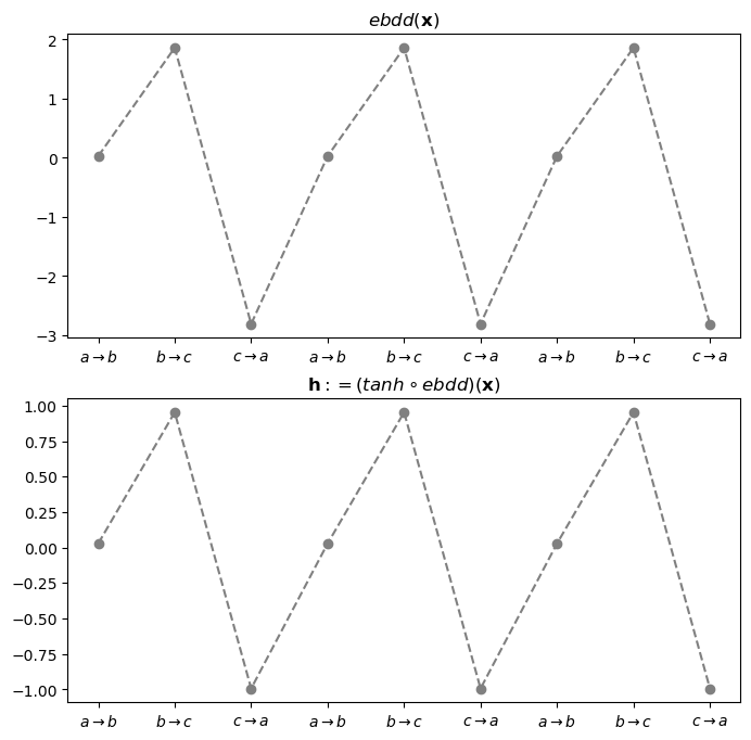

• 여기까지 2개는 세트로 보는 것이 좋겠다.
• 결과를 \(h\)로 생각하자.

- Ebdd -> tanh -> linr 통과직후 - 여기에서 차원이 3차원으로 된다.

ebdd_x = ebdd(x).data[:9]
h = tanh(ebdd(x)).data[:9]
netout = linr(tanh(ebdd(x))).data[:9]
#netout = net(x).data[:9]
torch.concat([ebdd_x,h,netout],axis=1)

tensor([[ 0.0287,  0.0287, -1.3637,  0.8247, -1.3384],
        [ 1.8616,  0.9528, -4.9139,  1.2273,  2.9339],
        [-2.8092, -0.9928,  2.5602,  0.3797, -6.0603],
        [ 0.0287,  0.0287, -1.3637,  0.8247, -1.3384],
        [ 1.8616,  0.9528, -4.9139,  1.2273,  2.9339],
        [-2.8092, -0.9928,  2.5602,  0.3797, -6.0603],
        [ 0.0287,  0.0287, -1.3637,  0.8247, -1.3384],
        [ 1.8616,  0.9528, -4.9139,  1.2273,  2.9339],
        [-2.8092, -0.9928,  2.5602,  0.3797, -6.0603]])

netout_a = netout[:,[0]]
netout_b = netout[:,[1]]
netout_c = netout[:,[2]]

linr.weight, linr.bias

(Parameter containing:
 tensor([[-3.8416],
         [ 0.4357],
         [ 4.6228]], requires_grad=True),
 Parameter containing:
 tensor([-1.2536,  0.8122, -1.4709], requires_grad=True))

netout_a, h*(-3.8416) + (-1.2536)

(tensor([[-1.3637],
         [-4.9139],
         [ 2.5602],
         [-1.3637],
         [-4.9139],
         [ 2.5602],
         [-1.3637],
         [-4.9139],
         [ 2.5602]]),
 tensor([[-1.3637],
         [-4.9140],
         [ 2.5602],
         [-1.3637],
         [-4.9140],
         [ 2.5602],
         [-1.3637],
         [-4.9140],
         [ 2.5602]]))

fig,ax = plt.subplots(2,1,figsize=(8,8))
ax[0].plot(h, '--o', color='gray')
ax[0].set_title(r"${\bf h}:=(tanh \circ ebdd)({\bf x})$")
ax[0].set_xticks(range(9),[r'$a\to b$', r'$b\to c$', r'$c\to a$']*3);
ax[1].plot(netout_a, '--o', label=r"$netout_a =  (-3.8416)\times {\bf h} + (-1.2536)$")
ax[1].plot(netout_b, '--o', label=r"$netout_b =  ( 0.4357)\times {\bf h} + (0.8122)$")
ax[1].plot(netout_c, '--o', label=r"$netout_c =  (4.6228)\times {\bf h} + (-1.4709)$")
ax[1].set_xticks(range(9),[r'$a\to b$', r'$b\to c$', r'$c\to a$']*3);
ax[1].legend()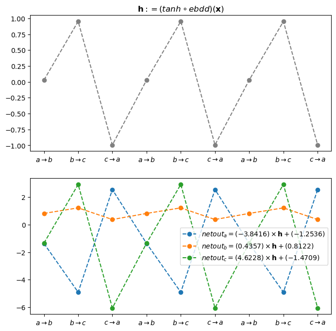

- 이 네트워크는 b->c 인 맵핑과 c->a인 맵핑은 확실하게 학습한 것 같지만 a->b인 맵핑은 그다지 잘 학습한 느낌이 들지 않는다.

- 전체과정 시각화

onehot_x = ohot(x).data[:9]
onehot_a = onehot_x[:,[0]]
onehot_b = onehot_x[:,[1]]
onehot_c = onehot_x[:,[2]]
#--#
ebdd_x = ebdd(x).data[:9]
#--#
h = tanh(ebdd(x)).data[:9]
#--#
netout = linr(tanh(ebdd(x))).data[:9]
netout_a = netout[:,[0]]
netout_b = netout[:,[1]]
netout_c = netout[:,[2]]
#--#
yhat = soft(net(x)).data[:9]
yhat_a = yhat[:,[0]]
yhat_b = yhat[:,[1]]
yhat_c = yhat[:,[2]]
#--#
torch.concat([ebdd_x,h,netout,yhat],axis=1).numpy().round(2)

array([[ 0.03,  0.03, -1.36,  0.82, -1.34,  0.09,  0.81,  0.09],
       [ 1.86,  0.95, -4.91,  1.23,  2.93,  0.  ,  0.15,  0.85],
       [-2.81, -0.99,  2.56,  0.38, -6.06,  0.9 ,  0.1 ,  0.  ],
       [ 0.03,  0.03, -1.36,  0.82, -1.34,  0.09,  0.81,  0.09],
       [ 1.86,  0.95, -4.91,  1.23,  2.93,  0.  ,  0.15,  0.85],
       [-2.81, -0.99,  2.56,  0.38, -6.06,  0.9 ,  0.1 ,  0.  ],
       [ 0.03,  0.03, -1.36,  0.82, -1.34,  0.09,  0.81,  0.09],
       [ 1.86,  0.95, -4.91,  1.23,  2.93,  0.  ,  0.15,  0.85],
       [-2.81, -0.99,  2.56,  0.38, -6.06,  0.9 ,  0.1 ,  0.  ]],
      dtype=float32)

fig, ax = plt.subplots(5,1,figsize=(8,16))
ax[0].set_title(r"$onehot({\bf x})$")
ax[0].set_xticks(range(9),[r'$a\to b$', r'$b\to c$', r'$c\to a$']*3)
ax[0].plot(onehot_a,'--o',label="a")
ax[0].plot(onehot_b,'--o',label="b")
ax[0].plot(onehot_c,'--o',label="c")
ax[0].legend()
#--#
ax[1].set_title(r"$ebdd({\bf x}):=(linr_{3 \to 1} \circ onehot)({\bf x})$")
ax[1].set_xticks(range(9),[r'$a\to b$', r'$b\to c$', r'$c\to a$']*3)
ax[1].plot(ebdd_x, '--o', color='gray')
#--#
ax[2].set_title(r"${\bf h}:=(tanh \circ ebdd)({\bf x})$")
ax[2].set_xticks(range(9),[r'$a\to b$', r'$b\to c$', r'$c\to a$']*3)
ax[2].plot(h, '--o', color='gray')
#--#
ax[3].set_title(r"$net({\bf x})=(linr_{1 \to 3} \circ tanh \circ ebdd)({\bf x})$")
ax[3].set_xticks(range(9),[r'$a\to b$', r'$b\to c$', r'$c\to a$']*3)
ax[3].plot(netout_a,'--o',label=r"$netout_a =  (-3.8416)\times {\bf h} + (-1.2536)$")
ax[3].plot(netout_b,'--o',label=r"$netout_b =  ( 0.4357)\times {\bf h} + (0.8122)$")
ax[3].plot(netout_c,'--o',label=r"$netout_c =  (4.6228)\times {\bf h} + (-1.4709)$")
ax[3].legend()
#--#
ax[4].set_title(r"$\hat{\bf y} = soft(net({\bf x}))$")
ax[4].set_xticks(range(9),[r'$a\to b$', r'$b\to c$', r'$c\to a$']*3)
ax[4].plot(yhat_a,'--o',label=r"$P_a$")
ax[4].plot(yhat_b,'--o',label=r"$P_b$")
ax[4].plot(yhat_c,'--o',label=r"$P_c$")
ax[4].legend()
plt.tight_layout()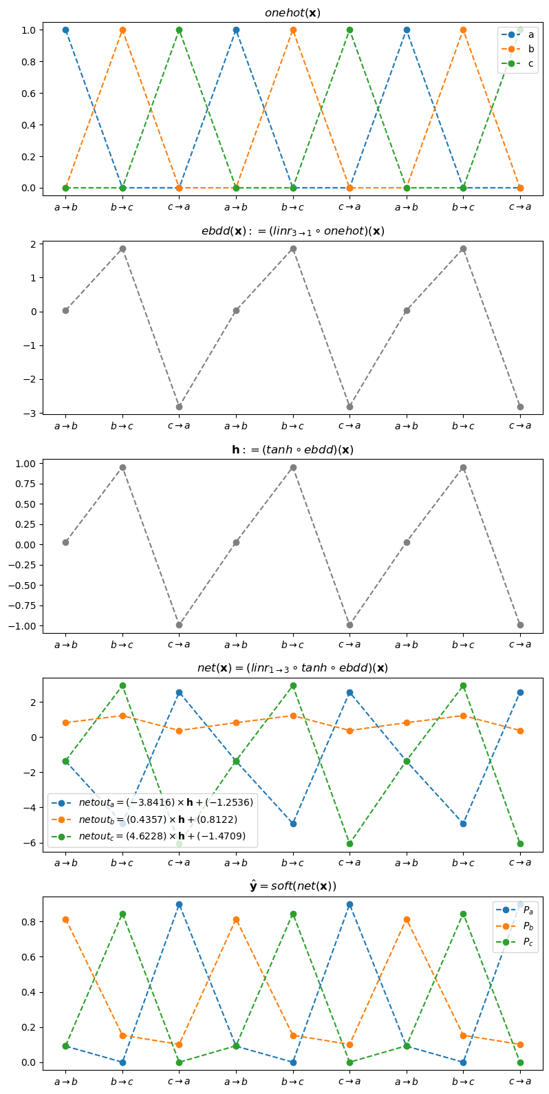

- 다른 방식의 시각화

h = tanh(ebdd(x)).data[:9]
netout = linr(tanh(ebdd(x))).data[:9]
yhat = soft(net(x)).data[:9]
mat = torch.concat([h,netout,yhat],axis=1)
#---#
plt.matshow(mat,cmap="bwr",vmin=-6,vmax=6)
plt.colorbar()
plt.axvline(0.5,color="lime")
plt.axvline(3.5,color="lime")
plt.xticks(ticks=[0,1,2,3,4,5,6],labels=[r"$h$",r"$out_a$",r"$out_b$",r"$out_c$",r"$P_a$",r"$P_b$",r"$P_c$"]);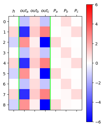

• \(h\)에 해당하는 색이 하얀색인 것이 있는데 이것은 b가 선택될 때 이런 일이 발생함. 이것은 값이 0이라는 의미인데 linr(3,1)에서 weight값은 0으로 되고 bias만 남는다는 의미이다. 그러므로 특징을 잡기가 불리하다.
• 따라서 \(h\)가 확실한 색을 가지고 있는 것이 유리하다. 그렇지만 확실한 색인 빨강과 파랑이 이미 차지된 상태라 어쩔 수 없이 0이 선택된 것이다.

D. MLP - 두개의 은닉노드

- 적합

torch.manual_seed(43052)
net = torch.nn.Sequential(
    torch.nn.Embedding(num_embeddings=3,embedding_dim=2), # 받아주는 차원이 2차원으로 늘어남
    torch.nn.Tanh(),
    torch.nn.Linear(in_features=2,out_features=3),
    #torch.nn.Softmax(),
)
loss_fn = torch.nn.CrossEntropyLoss() 
optimizr = torch.optim.Adam(net.parameters(),lr=0.1)

for epoc in range(50):
    ## 1 
    netout = net(x)
    ## 2 
    loss = loss_fn(netout,y)
    ## 3 
    loss.backward()
    ## 4 
    optimizr.step()
    optimizr.zero_grad()

- 결과 시각화

ebdd,tanh,linr = net
h = tanh(ebdd(x)).data[:9]
netout = linr(tanh(ebdd(x))).data[:9]
yhat = soft(net(x)).data[:9]
mat = torch.concat([h,netout,yhat],axis=1)
#---#
plt.matshow(mat,cmap="bwr",vmin=-6,vmax=6)
plt.colorbar()
plt.axvline(1.5,color="lime")
plt.axvline(4.5,color="lime")
plt.xticks(ticks=[0,1,2,3,4,5,6,7],labels=[r"$h_1$",r"$h_2$",r"$out_a$",r"$out_b$",r"$out_c$",r"$P_a$",r"$P_b$",r"$P_c$"]);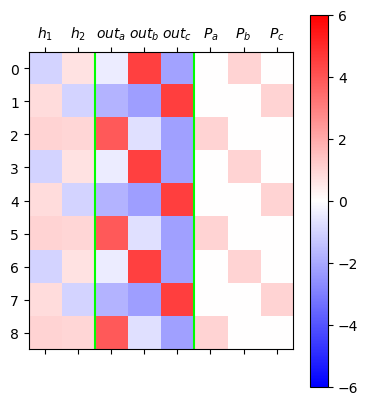

• x=a -> h = (파,빨) -> y=b
• x=b -> h = (빨,파) -> y=c
• x=c -> h = (빨,빨) -> y=a
• h=(파,파)는 아직 사용되지 않음. 즉 d를 하나 더 쓸 수 있는 공간이 남아있다는 의미이다.

3. abcd

A. Data

- d 하나 더 써보자.

txt = list('abcd'*100)
txt[:10]

['a', 'b', 'c', 'd', 'a', 'b', 'c', 'd', 'a', 'b']

df_train = pd.DataFrame({'x':txt[:-1], 'y':txt[1:]})
df_train[:5]

	x	y
0	a	b
1	b	c
2	c	d
3	d	a
4	a	b

x = torch.tensor(df_train.x.map({'a':0, 'b':1, 'c':2, 'd':3}))
y = torch.tensor(df_train.y.map({'a':0, 'b':1, 'c':2, 'd':3}))

B. MLP - 하나의 은닉노드

- 학습

net = torch.nn.Sequential(
    torch.nn.Embedding(num_embeddings=4,embedding_dim=1),
    torch.nn.Tanh(),
    torch.nn.Linear(in_features=1,out_features=4)
)
ebdd,tanh,linr = net 
ebdd.weight.data = torch.tensor([[-0.3333],[-2.5000],[5.0000],[0.3333]])
linr.weight.data = torch.tensor([[1.5000],[-6.0000],[-2.0000],[6.0000]])
linr.bias.data = torch.tensor([0.1500, -2.0000,  0.1500, -2.000])
loss_fn = torch.nn.CrossEntropyLoss()
optimizr = torch.optim.Adam(net.parameters(),lr=0.1)

for epoc in range(50):
    ## 1 
    netout = net(x)
    ## 2 
    loss = loss_fn(netout,y)
    ## 3 
    loss.backward()
    ## 4 
    optimizr.step()
    optimizr.zero_grad()

- 결과 시각화1

onehot_x = ohot(x).data[:8]
onehot_a = onehot_x[:,[0]]
onehot_b = onehot_x[:,[1]]
onehot_c = onehot_x[:,[2]]
onehot_d = onehot_x[:,[3]]
#--#
ebdd_x = ebdd(x).data[:8]
#--#
h = tanh(ebdd(x)).data[:8]
#--#
netout = linr(tanh(ebdd(x))).data[:8]
netout_a = netout[:,[0]]
netout_b = netout[:,[1]]
netout_c = netout[:,[2]]
netout_d = netout[:,[3]]
#--#
yhat = soft(net(x)).data[:8]
yhat_a = yhat[:,[0]]
yhat_b = yhat[:,[1]]
yhat_c = yhat[:,[2]]
yhat_d = yhat[:,[3]]
#--#

fig, ax = plt.subplots(5,1,figsize=(8,16))
ax[0].set_title(r"$onehot({\bf x})$")
ax[0].set_xticks(range(8),[r'$a\to b$', r'$b\to c$', r'$c\to d$', r'$d\to a$']*2)
ax[0].plot(onehot_a,'--o',label="a")
ax[0].plot(onehot_b,'--o',label="b")
ax[0].plot(onehot_c,'--o',label="c")
ax[0].plot(onehot_d,'--o',label="d")
ax[0].legend()
#--#
ax[1].set_title(r"$ebdd({\bf x})$")
ax[1].set_xticks(range(8),[r'$a\to b$', r'$b\to c$', r'$c\to d$', r'$d\to a$']*2)
ax[1].plot(ebdd_x, '--o', color='gray')
#--#
ax[2].set_title(r"${\bf h}:=(tanh \circ ebdd)({\bf x})$")
ax[2].set_xticks(range(8),[r'$a\to b$', r'$b\to c$', r'$c\to d$', r'$d\to a$']*2)
ax[2].plot(h, '--o', color='gray')
#--#
ax[3].set_title(r"$net({\bf x})=(linr \circ tanh \circ ebdd)({\bf x})$")
ax[3].set_xticks(range(8),[r'$a\to b$', r'$b\to c$', r'$c\to d$', r'$d\to a$']*2)
ax[3].plot(netout_a,'--o',label=r"$netout_a$")
ax[3].plot(netout_b,'--o',label=r"$netout_b$")
ax[3].plot(netout_c,'--o',label=r"$netout_c$")
ax[3].plot(netout_d,'--o',label=r"$netout_d$")
ax[3].legend()
#--#
ax[4].set_title(r"$\hat{\bf y} = soft(net({\bf x}))$")
ax[4].set_xticks(range(8),[r'$a\to b$', r'$b\to c$', r'$c\to d$', r'$d\to a$']*2)
ax[4].plot(yhat_a,'--o',label=r"$P_a$")
ax[4].plot(yhat_b,'--o',label=r"$P_b$")
ax[4].plot(yhat_c,'--o',label=r"$P_c$")
ax[4].plot(yhat_d,'--o',label=r"$P_d$")
ax[4].legend()
plt.tight_layout()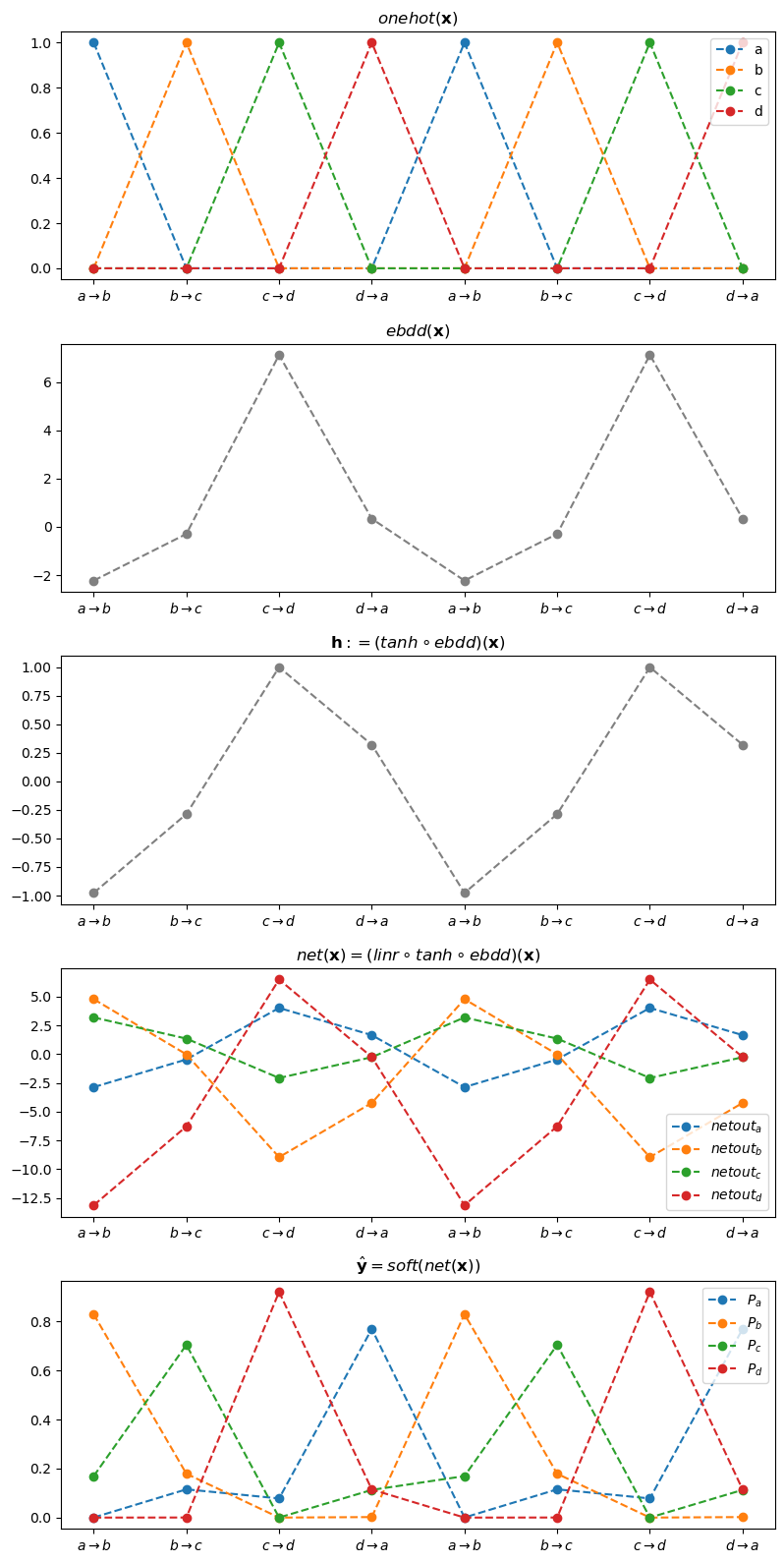

- 결과 시각화2

ebdd,tanh,linr = net
h = tanh(ebdd(x)).data[:8]
netout = linr(tanh(ebdd(x))).data[:8]
yhat = soft(net(x)).data[:8]
mat = torch.concat([h,netout,yhat],axis=1)
#---#
plt.matshow(mat,cmap="bwr",vmin=-6,vmax=6)
plt.colorbar()
plt.axvline(0.5,color="lime")
plt.axvline(4.5,color="lime")
plt.xticks(ticks=[0,1,2,3,4,5,6,7,8],labels=[r"$h$",r"$out_a$",r"$out_b$",r"$out_c$",r"$out_d$",r"$P_a$",r"$P_b$",r"$P_c$",r"$P_d$"]);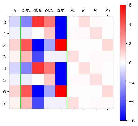

C. MLP - 두 개의 은닉노드

- 학습

torch.manual_seed(43052)
net = torch.nn.Sequential(
    torch.nn.Embedding(num_embeddings=4,embedding_dim=2),
    torch.nn.Tanh(),
    torch.nn.Linear(in_features=2,out_features=4)
)
loss_fn = torch.nn.CrossEntropyLoss()
optimizr = torch.optim.Adam(net.parameters(),lr=0.1)

for epoc in range(50):
    ## 1 
    netout = net(x)
    ## 2 
    loss = loss_fn(netout,y)
    ## 3 
    loss.backward()
    ## 4 
    optimizr.step()
    optimizr.zero_grad()

- 결과 시각화

ebdd,tanh,linr = net
h = tanh(ebdd(x)).data[:8]
netout = linr(tanh(ebdd(x))).data[:8]
yhat = soft(net(x)).data[:8]
mat = torch.concat([h,netout,yhat],axis=1)
#---#
plt.matshow(mat,cmap="bwr",vmin=-6,vmax=6)
plt.colorbar()
plt.axvline(1.5,color="lime")
plt.axvline(5.5,color="lime")
plt.xticks(ticks=range(10),labels=[r"$h_1$",r"$h_2$",r"$out_a$",r"$out_b$",r"$out_c$",r"$out_d$",r"$P_a$",r"$P_b$",r"$P_c$",r"$P_d$"]);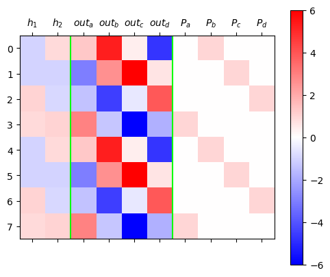

D. 비교실험

- 은닉노드 1개

class Net1(torch.nn.Module):
    def __init__(self):
        super().__init__()
        ## 우리가 yhat을 구할때 사용할 레이어를 정의 
        self.ebdd = torch.nn.Embedding(4,1)
        self.tanh = torch.nn.Tanh()
        self.linr = torch.nn.Linear(1,4)
        ## 정의 끝
    def forward(self,X):
        ## yhat을 어떻게 구할것인지 정의 
        ebdd_x = self.ebdd(x)
        h = self.tanh(ebdd_x)
        netout = self.linr(h)
        ## 정의 끝
        return netout

fig, ax = plt.subplots(5,5,figsize=(10,10))
for i in range(5):
    for j in range(5):
        net = Net1()
        optimizr = torch.optim.Adam(net.parameters(),lr=0.1)
        loss_fn = torch.nn.CrossEntropyLoss()
        for epoc in range(50):
            ## 1 
            netout = net(x)
            ## 2 
            loss = loss_fn(netout,y)
            ## 3 
            loss.backward()
            ## 4 
            optimizr.step()
            optimizr.zero_grad()
        h = net.tanh(net.ebdd(x)).data[:6]
        yhat = soft(net(x)).data[:6]
        mat = torch.concat([h,yhat],axis=1)
        ax[i][j].matshow(mat,cmap='bwr',vmin=-1,vmax=1)
        ax[i][j].axvline(0.5,color='lime')
        ax[i][j].set_xticks(ticks=[0,1,2,3,4],labels=[r"$h$",r"$P_a$",r"$P_b$",r"$P_c$",r"$P_d$"])
fig.suptitle("# of hidden nodes = 1", size=20)
fig.tight_layout()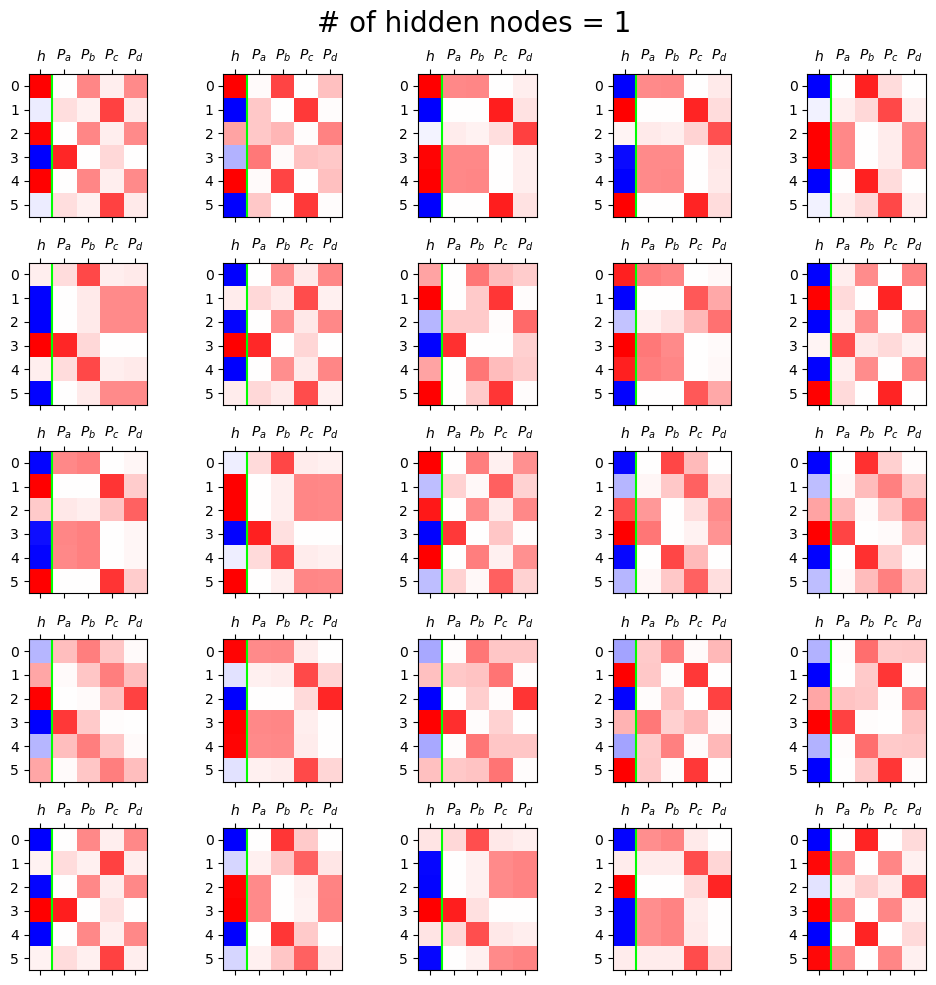

- 은닉노드 2개

class Net2(torch.nn.Module):
    def __init__(self):
        super().__init__()
        ## 우리가 yhat을 구할때 사용할 레이어를 정의 
        self.ebdd = torch.nn.Embedding(4,2)
        self.tanh = torch.nn.Tanh()
        self.linr = torch.nn.Linear(2,4)
        ## 정의 끝
    def forward(self,X):
        ## yhat을 어떻게 구할것인지 정의 
        ebdd_x = self.ebdd(x)
        h = self.tanh(ebdd_x)
        netout = self.linr(h)
        ## 정의 끝
        return netout

fig, ax = plt.subplots(5,5,figsize=(10,10))
for i in range(5):
    for j in range(5):
        net = Net2()
        optimizr = torch.optim.Adam(net.parameters(),lr=0.1)
        loss_fn = torch.nn.CrossEntropyLoss()
        for epoc in range(50):
            ## 1 
            netout = net(x)
            ## 2 
            loss = loss_fn(netout,y)
            ## 3 
            loss.backward()
            ## 4 
            optimizr.step()
            optimizr.zero_grad()
        h = net.tanh(net.ebdd(x)).data[:6]
        yhat = soft(net(x)).data[:6]
        mat = torch.concat([h,yhat],axis=1)
        ax[i][j].matshow(mat,cmap='bwr',vmin=-1,vmax=1)
        ax[i][j].axvline(1.5,color='lime')
        ax[i][j].set_xticks(ticks=[0,1,2,3,4,5],labels=[r"$h_1$",r"$h_2$",r"$P_a$",r"$P_b$",r"$P_c$",r"$P_d$"])
fig.suptitle("# of hidden nodes = 2", size=20)
fig.tight_layout()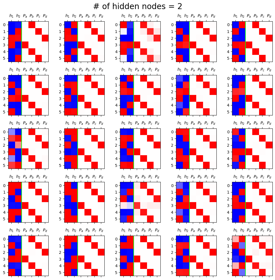        

5. \(h\)에 대하여

- \(h\)는 one_hot encoding보다 더 (1)액기스만 남은 느낌 + (2) 숙성된 느낌을 준다.

• (1)에 대한 내가 느낀 느낌은 one_hot encoding을 하면 위치정보로 a,b,c,d를 구분하는 느낌이다. 가중치를 곱해주면 a,b,c,d 따로따로 값이 들어가기 때문에 숫자정보도 있고 위치정보(a,b,c,d의 구분)도 담고 있어서 액기스만 남은 느낌을 준다.
• (2)에 대한 내가 느낀 느낌은 숙성된 느낌이라는 것은 epoc으로 오차를 재면서 고치고 또 고친 값들이다. 위치정보는 그대로이지만 숫자가 one_hot encoding보다 더 정교한 느낌이다.